


Things You Should Know Before Using Structural Equation Modeling.
Structural equation modeling (SEM) is a series of statistical methods that allow complex relationships between one or more independent variables and one or more dependent variables. Though there are many ways to describe SEM, it is most commonly thought of as a hybrid between some form of analysis of variance (ANOVA)/regression and some form of factor analysis. In general, it can be remarked that SEM allows one to perform some type of multilevel regression/ANOVA on factors. You should therefore be quite familiar with univariate and multivariate regression/ANOVA as well as the basics of factor analysis to implement SEM for your data.
Some preliminary terminology will also be useful. The following definitions regarding the types of variables that occur in SEM allow for a more clear explanation of the procedure:
- Variables that are not influenced by another variable in a model are called exogenous As an example, suppose we have two factors that cause changes in GPA, hours studying per week and IQ. Suppose there is no causal relationship between hours studying and IQ. Then both IQ and hours studying would be exogenous variables in the model.
- Variables that are influenced by other variables in a model are called endogenous GPA would be an endogenous variable in the previous example in (a).
- A variable that is directly observed and measured is called a manifest variable (it is also called an indicator variable in some circles). In the example in (a), all variables can be directly observed and thus qualify as manifest variables. There is a special name for a structural equation model that examines only manifest variables, called a path analysis.
- A variable that is not directly measured is latent The “factors” in factor analysis are latent variables. For example, suppose we were additionally interested in the impact of motivation on GPA. Motivation, as it is an internal, non-observable state, is indirectly assessed by a student’s response on a questionnaire, and thus it is a latent variable. Latent variables increase the complexity of a structural equation model because one needs to take into account all of the questionnaire items and measured responses that are used to quantify the “factor” or latent variable. In this instance, each item on the questionnaire would be a single variable that would either be significantly or insignificantly involved in a linear combination of variables that influence the variation in the latent factor of motivation
- For the purposes of SEM, specifically, moderation refers to a situation that includes three or more variables, such that the presence of one of those variables changes the relationship between the other two. In other words, moderation exists when the association between two variables is not the same at all levels of a third variable. One way to think of moderation is when you observe an interaction between two variables in an ANOVA. For example, stress and psychological adjustment may differ at different levels of social support (i.e., this is the definition of an interaction). In other words, stress may adversely affect adjustment more under conditions of low social support compared to conditions of high social support. This would imply a two-way interaction between stress and psychological support if an ANOVA were to be performed. Figure 1 shows a conceptual diagram of moderation. This diagram shows that there are three direct effects that are hypothesized to cause changes in psychological adjustment – the main effect of stress, the main effect of social support, and an interaction effect of stress and social support.
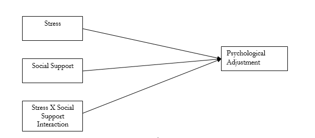
Figure 1. A Diagrammed Example of Moderation. Note that each individual effect of stress, social support, and the interaction of stress and social support can be separated and is said to be related to psychological adjustment. Also, note that there are no causal connections between stress and social support.
6. For the purposes of SEM, specifically, mediation refers to a situation that includes three or more variables, such that there is a causal process between all three variables. Note that this is distinct from moderation. In the previous example in (e), we can say there are three separate things in the model that cause a change in psychological adjustment: stress, social support, and the combined effect of stress and social support that is not accounted for by each individual variable. Mediation describes a much different relationship that is generally more complex. In a mediation relationship, there is a direct effect between an independent variable and a dependent variable. There are also indirect effects between an independent variable and a mediator variable, and between a mediator variable and a dependent variable. The example in (e) above can be re-specified into a mediating process, as shown in Figure 2 below. The main difference from the moderation model is that we now allow for causal relationships between stress and social support and social support and psychological adjustment to be expressed. Imagine that social support was not included in the model – we just wanted to see the direct effect of stress and psychological adjustment. We would get a measure of the direct effect by using regression or ANOVA. When we include social support as a mediator, that direct effect will change as a result of decomposing the causal process into indirect effects of stress on social support and social support on psychological adjustment. The degree to which the direct effect changes as a result of including the mediating variable of social support is referred to as the mediational effect. Testing for mediation involves running a series of regression analyses for all of the causal pathways and some method of estimating a change indirect effect. This technique is actually involved in structural equation models that include mediator variables and will be discussed in the next section of this document.
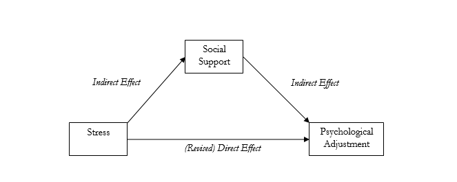
Figure 2. A Diagram of a Mediation Model. Including indirect effects in a mediation model may change the direct effect of a single independent variable on a dependent variable.
In many respects, moderation and mediational models are the foundation of structural equation modeling. In fact, they can be considered as simple structural equation models themselves. Therefore, it is very important to understand how to analyze such models to understand more complex structural equation models that include latent variables. Generally, a mediation model like the one above can be implemented by doing a series of separate regressions. As described in later sections of this document, the effects in a moderation model can be numerically described by using path coefficients, which are identical or similar to regression coefficients, depending on the specific choice of analysis you are performing.
7. Covariance and correlation are the building blocks of how your data will be represented when doing any programming or model specification within a software program that implements structural equation modeling. You should know how to obtain a correlation matrix or covariance matrix using PROC CORR in SAS, or use other menu tools from a statistical package of your choice, to specify that a correlation or covariance matrix be calculated. The covariance matrix in practice serves as your dataset to be analyzed. In the context of SEM, covariances and correlations between variables are essential because they allow you to include a relationship between two variables that is not necessarily causal. In practice, most structural equation models contain both causal and non-causal relationships. Obtaining covariance estimates between variables allows one to better estimate direct and indirect effects with other variables, particularly in complex models with many parameters to be estimated.
8. A structural model is a part of the entire structural equation model diagram that you will complete for every model you propose. It is used to relate all of the variables (both latent and manifest) you will need to account for in the model. There are a few important rules to follow when creating a structural model and they will be discussed in the second section of this document.
9. A measurement model is a part of the entire structural equation model diagram that you will complete for every model you propose. It is essential if you have latent variables in your model. This part of the diagram which is analogous to factor analysis: You need to include all individual items, variables, or observations that “load” onto the latent variable, their relationships, variances, and errors. There are a few important rules to follow when creating the measurement model and they will be discussed in the second section of this document.
10. Together, the structural model and the measurement model form the entire structural equation model. This model includes everything that has been measured, observed, or otherwise manipulated in the set of variables examined.
11. A recursive structural equation model is a model in which causation is directed in one single direction. A nonrecursive structural equation model has causation which flows in both directions at some parts of the model.
Types of Research Questions Answered by SEM
SEM can conceptually be used to answer any research question involving the indirect or direct observation of one or more independent variables or one or more dependent variables. However, the primary goal of SEM is to determine and validify a proposed causal process and/or model. Therefore, SEM is a confirmatory technique. Like any other test or model, we have a sample and want to say something about the population that comprises the sample. We have a covariance matrix to serve as our dataset, which is based on the sample of collected measurements. The empirical question of SEM is therefore whether the proposed model produces a population covariance matrix that is consistent with the sample covariance matrix. Because one must specify a priori a model that will undergo validation testing, there are many questions SEM can answer.
SEM can tell you how if your model is adequate or not. Parameters are estimated and compared with the sample covariance matrix. The goodness of fit statistics can be calculated that will tell you whether your model is appropriate or needs further revision. SEM can also be used to compare multiple theories that are specified a priori.
SEM can tell you the amount of variance in the dependent variables (DVs) – both manifest and latent DVs – is accounted for by the IVs. It can also tell you the reliability of each measured variable. And, as previously mentioned, SEM allows you to examine mediation and moderation, which can include indirect effects.
SEM can also tell you about group differences. You can fit separate structural equation models for different groups and compare results. In addition, you can include both random and fixed effects in your models and thus include hierarchical modeling techniques in your analyses.
Limitations and Assumptions Regarding SEM
Because SEM is a confirmatory technique, you must plan accordingly. You must specify a full model a priori and test that model based on the sample and variables included in your measurements. You must know the number of parameters you need to estimate – including covariances, path coefficients, and variances. You must know all relationships you want to specify in the model. Then, and only then, can you begin your analyses?
Because SEM has the ability to model complex relationships between multivariate data, the sample size is an important (but unfortunately underemphasized) issue. Two popular assumptions are that you need more than 200 observations, or at least 50 more than 8 times the number of variables in the model. Larger sample size is always desired for SEM.
Like other multivariate statistical methodologies, most of the estimation techniques used in SEM require multivariate normality. Your data need to be examined for univariate and multivariate outliers. Transformations on the variables can be made. However, there are some estimation methods that do not require normality.
SEM techniques only look at first-order (linear) relationships between variables. Linear relationships can be explored by creating bivariate scatterplots for all of your variables. Power transformations can be made if a relationship between two variables seems quadratic.
Multicollinearity among the IVs for manifest variables can be an issue. Most programs will inspect the determinant of a section of your covariance matrix or the whole covariance matrix. A very small determinant may be indicative of extreme multicollinearity.
The residuals of the covariances (not residual scores) need to be small and centered about zero. Some goodness of fit tests (like the Lagrange Multiplier test) remains robust against highly deviated residuals or non-normal residuals.
Preparing Your Data for Analysis
Assuming you have checked for model assumptions, dealt with missing data, and imported your data into a software package, you should obtain a covariance matrix on your dataset. In SAS, you can run PROC CORR and create an output file that has the covariance matrix. Alternatively, you can manually type in the covariance matrix or import it from a spreadsheet. You must specify in the data declaration that the set is a covariance matrix, so, in SAS for example, your code would appear as data-name type=COV; effort must be made to ensure the decimals of the entries are aligned. Other programs like EQS or LISREL can handle full datasets and will automatically compute covariance matrices for you.
Developing the Model Hypothesis and Model Specification
Often, the most difficult part of SEM is correctly identifying your model. You must know exactly the number of latent and manifest variables you are including in your model, as well as the number of variances and covariances to be calculated, as well as the number of parameters you are estimating. This section details the rules and conventions that are used when specifying a model. At this time it does not cover a complete set of rules for each popular software programs that are available (EQS, LISREL, AMOS, and PROC CALIS in SAS). In general, though, the conventions that follow are generally compatible with the existing software programs.
Drawing your hypothesized model: procedures and notation
The most important part of SEM analysis is the causal model you are required to draw before attempting an analysis. The following basic, general rules are used when drawing a model:
Rule 1. Latent variables/factors are represented with circles and measured/manifest variables are represented with squares.
Rule 2. Lines with an arrow in one direction show a hypothesized direct relationship between the two variables. It should originate at the causal variable and point to the variable that is caused. The absence of a line indicates there is no causal relationship between the variables.
Rule 3. Lines with an arrow in both directions should be curved and this demonstrates a bi-directional relationship (i.e., a covariance).
Rule 3a. Covariance arrows should only be allowed for exogenous variables.
Rule 4. For every endogenous variable, a residual term should be added to the model. Generally, a residual term is a circle with the letter E written in it, which stands for error.
Rule 4a. For latent variables that are also endogenous, a residual term is not called error in the lingo of SEM. It is called a disturbance, and therefore the “error term” here would be a circle with a D written in it, standing for the disturbance.
These rules need to be expanded and completed. An example diagram (that is analyzed later on) is included on the next page.


")


")
