


Below article given an example of CFA model with Latent Variable Analysis (Lavaan) in R.
We start with a simple example of confirmatory factor analysis, using the cfa() function, which is a user-friendly function for fitting CFA models. The lavaan package contains a built-in dataset called HolzingerSwineford1939. See the help page for this dataset by typing
?HolzingerSwineford1939
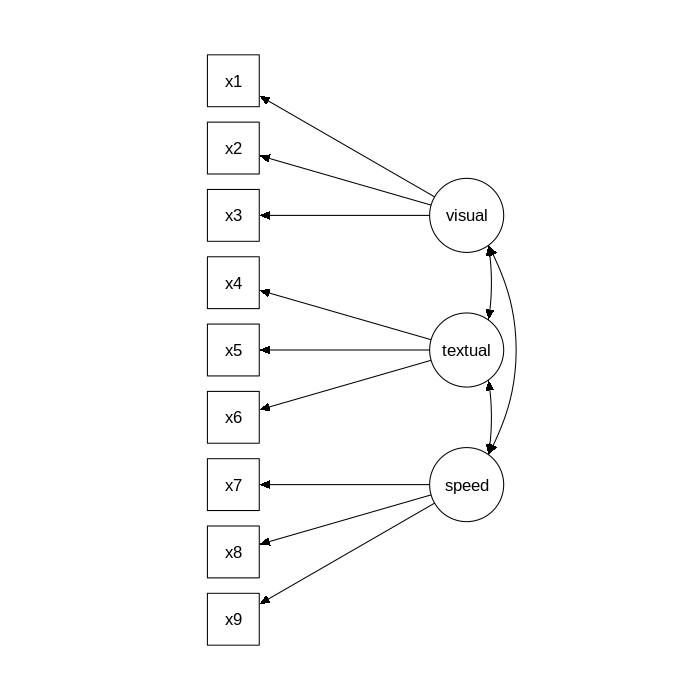
at the R prompt. This is a ‘classic’ dataset that is used in many papers and books on Structural Equation Modeling (SEM), including some manuals of commercial SEM software packages. The data consists of mental ability test scores of seventh- and eighth-grade children from two different schools (Pasteur and Grant-White). In our version of the dataset, only 9 out of the original 26 tests are included. A CFA model that is often proposed for these 9 variables consists of three latent variables (or factors), each with three indicators:
- a visual factor measured by 3 variables:
x1,x2andx3 - a textual factor measured by 3 variables:
x4,x5andx6 - a speed factor measured by 3 variables:
x7,x8andx9
The figure below contains a graphical representation of the three-factor model.
The corresponding lavaan syntax for specifying this model is as follows:
 visual =~ x1 + x2 + x3
textual =~ x4 + x5 + x6
  speed =~ x7 + x8 + x9
In this example, the model syntax only contains three ‘latent variable definitions’. Each formula has the following format:
latent variable =~ indicator1 + indicator2 + indicator3
We call these expressions latent variable definitions because they define how the latent variables are ‘manifested by’ a set of observed (or manifest) variables, often called ‘indicators’. Note that the special “=~" operator in the middle consists of a sign (“=“) character and a tilde ("~") character next to each other. The reason why this model syntax is so short, is that behind the scenes, the function will take care of several things. First, by default, the factor loading of the first indicator of a latent variable is fixed to 1, thereby fixing the scale of the latent variable. Second, residual variances are added automatically. And third, all exogenous latent variables are correlated by default. This way, the model syntax can be kept concise. On the other hand, the user remains in control, since all this ‘default’ behavior can be overriden and/or switched off.
We can enter the model syntax using the single quotes:
HS.model <- ' visual  =~ x1 + x2 + x3
              textual =~ x4 + x5 + x6
              speed   =~ x7 + x8 + x9 '
We can now fit the model as follows:
fit <- cfa(HS.model, data=HolzingerSwineford1939)
The cfa() function is a dedicated function for fitting confirmatory factor analysis models. The first argument is the user-specified model. The second argument is the dataset that contains the observed variables. Once the model has been fitted, the summary() function provides a nice summary of the fitted model:
summary(fit, fit.measures=TRUE)
The output should look familiar to users of other SEM software. If you find it confusing or esthetically unpleasing, please let us know, and we will try to improve it.
lavaan (0.6-1) converged normally after  35 iterations

  Number of observations                           301

  Estimator                                         ML
  Model Fit Test Statistic                      85.306
  Degrees of freedom                                24
  P-value (Chi-square)                           0.000

Model test baseline model:

  Minimum Function Test Statistic              918.852
  Degrees of freedom                                36
  P-value                                        0.000

User model versus baseline model:

  Comparative Fit Index (CFI)                    0.931
  Tucker-Lewis Index (TLI)                       0.896

Loglikelihood and Information Criteria:

  Loglikelihood user model (H0)              -3737.745
  Loglikelihood unrestricted model (H1)      -3695.092

  Number of free parameters                         21
  Akaike (AIC)                                7517.490
  Bayesian (BIC)                              7595.339
  Sample-size adjusted Bayesian (BIC)         7528.739

Root Mean Square Error of Approximation:

  RMSEA                                          0.092
  90 Percent Confidence Interval          0.071  0.114
  P-value RMSEA <= 0.05                          0.001

Standardized Root Mean Square Residual:

  SRMR                                           0.065

Parameter Estimates:

  Information                                 Expected
  Information saturated (h1) model          Structured
  Standard Errors                             Standard

Latent Variables:
                   Estimate  Std.Err  z-value  P(>|z|)
  visual =~
    x1                1.000
    x2                0.554    0.100    5.554    0.000
    x3                0.729    0.109    6.685    0.000
  textual =~
    x4                1.000
    x5                1.113    0.065   17.014    0.000
    x6                0.926    0.055   16.703    0.000
  speed =~
    x7                1.000
    x8                1.180    0.165    7.152    0.000
    x9                1.082    0.151    7.155    0.000

Covariances:
                   Estimate  Std.Err  z-value  P(>|z|)
  visual ~~
    textual           0.408    0.074    5.552    0.000
    speed             0.262    0.056    4.660    0.000
  textual ~~
    speed             0.173    0.049    3.518    0.000

Variances:
                   Estimate  Std.Err  z-value  P(>|z|)
   .x1                0.549    0.114    4.833    0.000
   .x2                1.134    0.102   11.146    0.000
   .x3                0.844    0.091    9.317    0.000
   .x4                0.371    0.048    7.779    0.000
   .x5                0.446    0.058    7.642    0.000
   .x6                0.356    0.043    8.277    0.000
   .x7                0.799    0.081    9.823    0.000
   .x8                0.488    0.074    6.573    0.000
   .x9                0.566    0.071    8.003    0.000
    visual            0.809    0.145    5.564    0.000
    textual           0.979    0.112    8.737    0.000
    speed             0.384    0.086    4.451    0.000
The output consists of three parts. The first six lines are called the header. The header contains the following information:
- the lavaan version number
- did lavaan converge normally or not, and how many iterations were needed
- the number of observations that were effectively used in the analysis
- the estimator that was used to obtain the parameter values (here:
ML) - the model test statistic, the degrees of freedom, and a corresponding p-value
The next section contains additional fit measures, and is only shown because we use the optional argument fit.measures = TRUE. It starts with the line Model test baseline model and ends with the value for the SRMR. The last section contains the parameter estimates. It starts with information about the standard errors (if the information matrix is expected or observed, and if the standard errors are standard, robust, or based on the bootstrap). Then, it tabulates all free (and fixed) parameters that were included in the model. Typically, first the latent variables are shown, followed by covariances and (residual) variances. The first column (Estimate) contains the (estimated or fixed) parameter value for each model parameter; the second column (Std.err) contains the standard error for each estimated parameter; the third column (Z-value) contains the Wald statistic (which is simply obtained by dividing the parameter value by its standard error), and the last column (P(>|z|)) contains the p-value for testing the null hypothesis that the parameter equals zero in the population.
To wrap up this first example, we summarize the complete code that was needed to fit this three-factor model:
# load the lavaan package (only needed once per session)
library(lavaan)

# specify the model
HS.model <- ' visual  =~ x1 + x2 + x3
              textual =~ x4 + x5 + x6
              speed   =~ x7 + x8 + x9 '

# fit the model
fit <- cfa(HS.model, data=HolzingerSwineford1939)

# display summary output
summary(fit, fit.measures=TRUE)
Simply copying this code and pasting it in R should work. The syntax illustrates the typical workflow in the lavaan package:
- Specify your model using the lavaan model syntax. In this example, only latent variable definitions have been used. In the following examples, other formula types will be used.
- Fit the model. This requires a dataset containing the observed variables (or alternatively the sample covariance matrix and the number of observations). In this example, we have used the
cfa()function. Other funcions in the lavaan package aresem()andgrowth()for fitting full structural equation models and growth curve models respectively. All three functions are so-called user-friendly functions, in the sense that they take care of many details automatically, so we can keep the model syntax simple and concise. If you wish to fit non-standard models or if you don’t like the idea that things are done for you automatically, you can use the lower-level functionlavaan()instead, where you have full control. - Extract information from the fitted model. This can be a long verbose summary, or it can be a single number only (say, the RMSEA value). In the spirit of R, you only get what you asked for. We try to not print out unnecessary information that you would ignore anyway.
Source: http://lavaan.ugent.be/tutorial/cfa.html


")


 Nginx with Let’s Encrypt on Ubuntu (Cloud VM, GCP, AWS, Azure, Linode) and Add Domain")


")
")